
Institut für Integrierte Systeme
Integrated Systems Laboratory
Neural Network Deeployment on the PULP Platform
Author: Victor J.B Jung
Date: 27th May 2025
Installation
⚠️ DISCLAIMER: The current container and commit are from main and devel, they will be tagged in the next release
Clone Deeploy and its submodules:
git clone https://github.com/pulp-platform/Deeploy.git && cd Deeploy
git submodule update --init --recursive
Pull the docker image:
docker pull ghcr.io/pulp-platform/deeploy:main
Run the container and bind Deeploy’s folder in the container:
docker run -it --name deeploy_main -v $(pwd):/app/Deeploy ghcr.io/pulp-platform/deeploy:main
Install Deeploy inside the container:
cd Deeploy
pip install -e .
From the DeeployTest folder, you can use the deeployRunner to compile ONNXs and execute the output code using the appropriate simulators.
To validate your installation, you can run a simple Add node on each platform:
python deeployRunner_generic.py -t Tests/Kernels/Integer/Add/Regular
python deeployRunner_cortexm.py -t Tests/Kernels/Integer/Add/Regular
python deeployRunner_mempool.py -t Tests/Kernels/Integer/Add/Regular
python deeployRunner_snitch.py -t Tests/Kernels/Integer/Add/Regular
python deeployRunner_siracusa.py -t Tests/Kernels/Integer/Add/Regular --cores=8
Once all these basic tests are passed, we can jump into the basics of Deeploy.
Deeploy 101
Deeploy is a compiler that transforms static computational graph (represented with the ONNX format) into bare-metal and (hopefully) optimized C. More specifically, it generates an application that can be deployed on the desired platform.
Hence, Deeploy’s inputs are:
An ONNX file describing your neural network.
Input tensors.
Expected output tensors generated with your favorite framework (ONNXRuntime or Torch, for instance).
Deeploy is shipped with a comprehensive testing framework conveniently named DeeployTest. This testing framework contains Test Runners for end-to-end testing of your network on a given platform. More specifically, a Test Runner compiles a given ONNX file, builds the project, feeds the inputs into the compiled neural network, and compares the output with the golden values to ensure correctness.
If you followed this tutorial correctly, you already used Test Runners (e.g., deeployRunner_siracusa.py) to validate the Deeploy installation! We will dive into the details of the Test Runners CLI very soon, but first, let’s look at the tools and libraries used downstream in Deeploy.
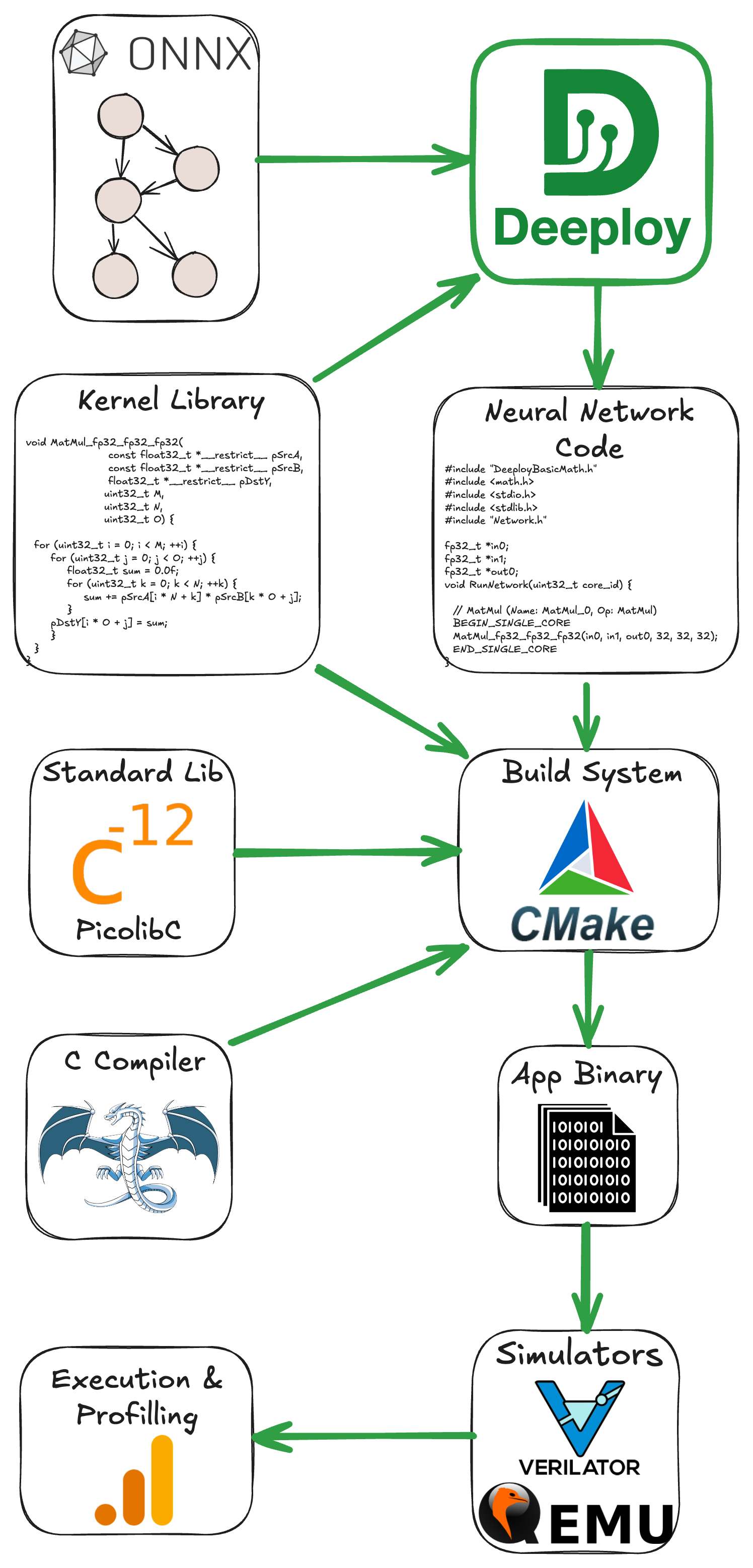
The figure below gives an overview of the deployment stack. As you can see, there are several steps to take before actually running the application. For the build system (e.g., the tool to organize compilation and linking), we use CMake. The default C compiler shipped with Deeploy is LLVM 15, but it supports GCC, given that you provide a local installation. To generate the Application Binary, we link the Network Code with the necessary Kernel Libraries and a Standard C Library (here Picolibc). Then, we feed this Application Binary to the appropriate simulator; from there, you can verify the correctness and benchmark the application.
You can visualize the ONNX graphs using Netron. Either use the web interface or install the python package with pip install netron.
✅ Task: Visualize the ONNX graph of the
Tests/Kernels/Integer/Add/Regular,Tests/Models/MobileNetv2, andTests/Models/Transformer
The ONNX graphs are in DeeployTest/Tests/<TestName>/network.onnx. The networks are increasing in complexity, Tests/Kernels/Integer/Add/Regular is a single node network for unit testing, while Tests/Models/MobileNetv2 is a simple sequential network mostly made of convolutions. Finally, the Tests/Models/Transformer network showcases a typical transformer block used in Encoder and Decoder networks. If you want to peek at a complex network, you can visualize Models/microLlama/microLlama128.
Now that we understand Deeploy’s input, let’s check the output-generated code!
✅ Task: Take a look at the code generated by Deeploy for the Generic platform.
The generated code is located in the following directory: DeeployTest/TEST_<PlatformName>/Tests, and the Network.c file is the interesting one.
The generated code is trivial for the Tests/Kernels/Integer/Add/Regular graph; we simply use the template for the Add node of the Generic platform. You can find the template declaration in Deeploy/Targets/Generic/Templates/AddTemplate.py.
Now, if you want to look at something a bit more complex, run python deeployRunner_generic.py -t ./Tests/Models/miniMobileNetv2 (from DeeployTest) and look at the generated code. There are two interesting points you can notice:
We hoist the constants at the top of the file.
In the
RunNetworkfunction, we sequentially have node templates to execute the operands and malloc/free to manage the memory. You can open the ONNX graph ofTests/Models/miniMobileNetv2on the side to try to match the nodes of the graph with their generated code.
✅ Task: Visualize the effect of passes on the ONNX graph for the Siracusa platform.
Deeploy applies passes on the ONNX graph to transform its topology and optimize its execution. Let’s visualize the effect of the passes used in the Siracusa Platform. First, let’s execute our miniMobileNetv2 on Siracusa with python deeployRunner_siracusa.py -t ./Tests/Models/miniMobileNetv2. You can find the original ONNX graph at Tests/Models/miniMobileNetv2/network.onnx, and the transformed ONNX graph at TEST_SIRACUSA/Tests/Models/miniMobileNetv2/deeployStates/backend_post_binding.onnx. Open both ONNX graphs side by side to compare them.
You can notice the effect of two passes on the graph:
One pass fuses the
ConvandRequantShiftnodes. This is a common technique named Operator Fusion and used in many DNN compilers.Another pass is adding a
Transposenode before theRequantizedConvin order to align the tensor layout from CHW to HWC (where C = Channels, H = Height, and W = Width). The HWC tensor layout is required to use optimized Convolution kernels (to learn more, check out this blog post).
Now that you understand the basics of Deeploy let’s jump into the optimized deployment of a small language model on the Siracusa SoC.
Micro Llama on Siracusa
Transformers 101
In this section, we will study the optimization of the deployment of a small language model. To fully understand this section, you need some basic understanding of Transformer’s architecture and Language Model inference mode. If you need a refresher on Transformer’s architecture, check out the Transformer Basics section of Lilian Weng’s blog post.
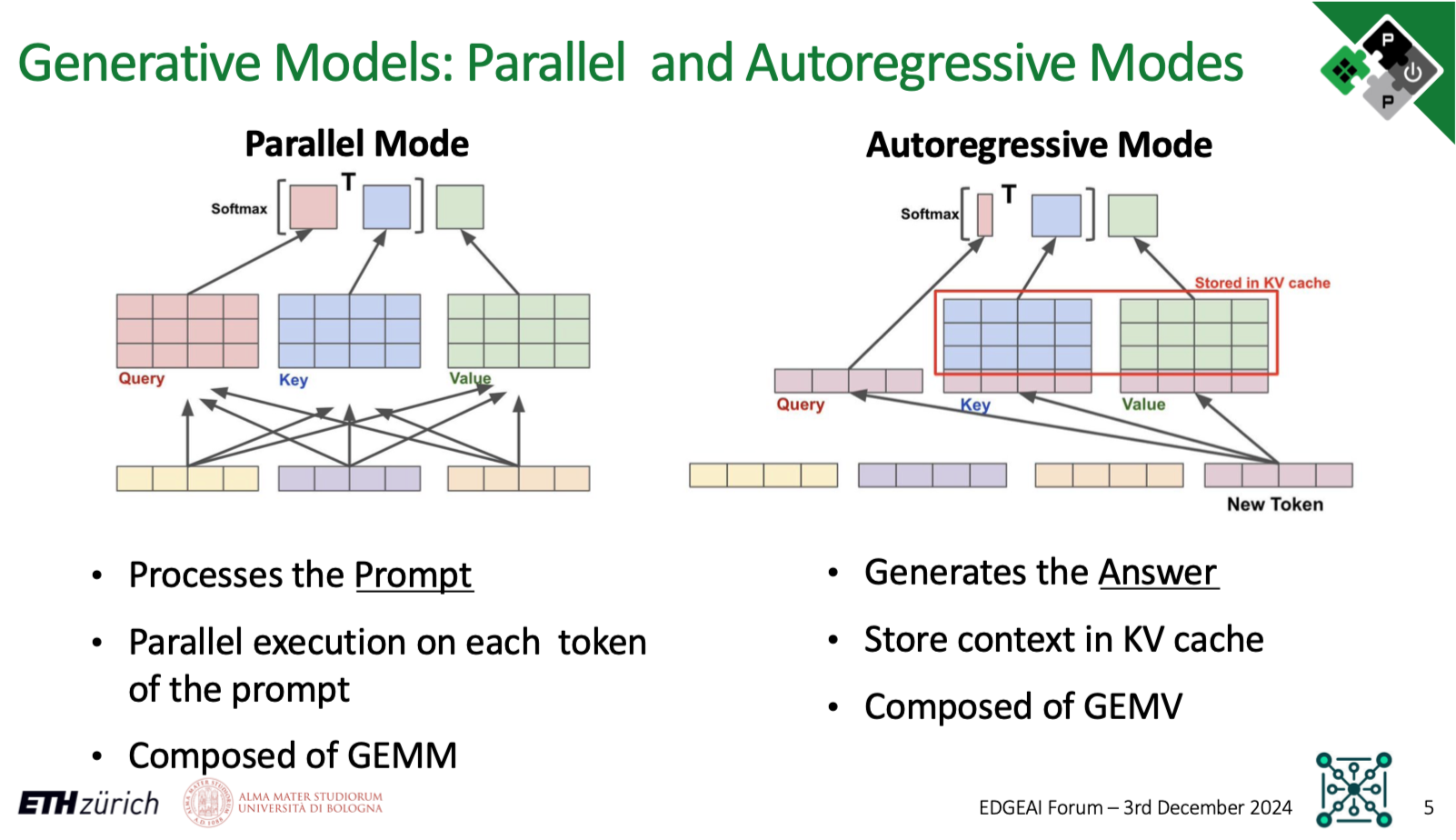
Now, Language Models have two inference modes:
The Parallel Mode (AKA Prefill Mode) is used to process the tokens of the prompts in parallel and generate the KV cache of the prompt and the first token of the Language Model’s “reply”. This mode contains mostly GEMMs.
The Autoregressive Mode generates the rest of the Language Model’s reply. It uses the KV cache from the previous step, generates a new KV cache entry, and predicts the next token. This mode contains mostly GEMVs.
To summarize, to generate a Language Model reply of \(N\) tokens, there is:
One Parallel Mode inference to process the prompt and generate the first token.
\(N-1\) Autoregressive Mode inferences to generate the rest of the tokens.
The slide below visually represents the Parallel Mode and Autoregressive Mode.
The Siracusa Platform
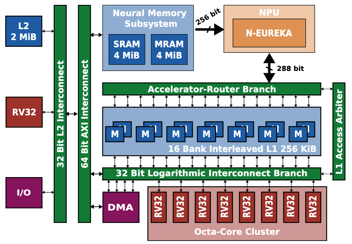
Let’s also quickly refresh our knowledge of the Siracusa platform to understand what kind of hardware we must deploy on. Below is the high-level block diagram of Siracusa, compute-wise we will mainly use:
The cluster of RV32 cores, they are modified to be great at crunching numbers. They feature SIMD, hardware loops (see the RI5CY user manual, p17), and the XPULP ISA extensions.
The NEUREKA NPU, an accelerator targeting integer convolutions.
In terms of memories, we have:
L3: An off-chip RAM (not shown on the block diagram) of 16MB capacity. The L3 has its own DMA that can transfer data to L2.
Neural Memory Subsystem (NMS): An SRAM/MRAM-based Weight Memory to store constants with a direct link to the NPU.
L2: An on-chip SRAM-based L2 memory of 2MB.
L1: A TCDM memory of size 256KB.
The on-chip DMA indicated on the block diagram can transfer data between the Weight Memory, the L2, and the L1.
Now that you understand the hardware and the kind of workload we want to execute. Let’s deploy using various optimizations to study their impact. The first parameter we can play with is the number of cores from the RV32 cluster to use.
✅ Task: Measure and compare the runtime of the
microLlama128model using 1 and 8 cores. Compute the speedup ratio; why is it not 8?
Hint: python deeployRunner_siracusa.py --help will list and explain the available flags.
Solution
If you run
python deeployRunner_siracusa.py -t Tests/Models/microLlama/microLlama128 --cores=1and thenpython deeployRunner_siracusa.py -t Tests/Models/microLlama/microLlama128 --cores=8, you should measure a runtime of ~16,1M cycles for 1 core and 3.1M cycles for 8 cores.The speedup ratio is obtained via \(\frac{\text{Runtime 1 cores}}{\text{Runtime 8 cores}} = 5.2\). Hence, using 8 cores instead of 1 leads to a 5.2 times speedup.
So why is the speedup ratio below 8? Mostly because all data movement is not overlapped with computation. Additionally, some kernels are probably not optimally parallelized for this specific network.
Tiling Basics
It’s due time to talk about data movement now! We use all 8 cluster cores, which is great, but where do these cores fetch the data from? By default, when using deeployRunner_siracusa.py, all data is in L2; there is no tiling, and cores read and write data directly to/from L2. As the L2 memory is “further away” from the cluster, load/store takes several cycles, which is non-optimal.
What we really want is to use the L1 memory, which provides 1 cycle latency load/store! But as the capacity is relatively small (256KB), we need to tile our layers. Tiling operands for an accelerator featuring only scratchpad memories is not trivial (unlike in architectures with data caches). For each layer, the compiler has to decide on tile size, a tiling schedule, a buffering strategy (single buffer, double buffer, etc…), and a memory allocation strategy. Then, the compiler must generate the code to configure and launch each transfer and place barriers accordingly to maximize concurrency.
The good news is that Deeploy can already do that! So, let’s generate and run some tiled code to see the impact of tiling on the runtime.
✅ Task: Get familiar with the CLI arguments of
deeployRunner_tiled_siracusa.py, then runmicroLlama64_parallelwith different configurations. Find one “bad” and one “good” configuration, and explain why.
Hint: Use the --help flag to list and explain the available flags.
Solution
Bad configuration:
python deeployRunner_tiled_siracusa.py -t Tests/Models/microLlama/microLlama64_parallel --cores=8 --l1 8000 --defaultMemLevel=L2-> Runtime: 47.5 MCyclesGood configuration
python deeployRunner_tiled_siracusa.py -t Tests/Models/microLlama/microLlama64_parallel --cores=8 --l1 64000 --defaultMemLevel=L2: -> Runtime: 35.3 MCyclesJustification: As the size of the L1 memory gets smaller, tiles also get smaller and smaller. Smaller tiles usually mean that it’s harder to keep the core properly utilized.
Profiling the Execution
To measure the effect of some optimizations in more detail, you can use the --profileTiling=L2 flag. This flag will enable a code transformation that will insert print displaying the runtime of several critical code sections. For instance, profiling an Integer Layer Normalization layer from L2 with two tiles will return the print the following:
[INTEGER_RMSNORM L2][SB][0 ops][Tile 0] Input DMA took 489 cycles
[INTEGER_RMSNORM L2][SB][0 ops][Tile 0] Kernel took 43305 cycles
[INTEGER_RMSNORM L2][SB][0 ops][Tile 0] Output DMA took 534 cycles
[INTEGER_RMSNORM L2][SB][0 ops][Tile 1] Input DMA took 82 cycles
[INTEGER_RMSNORM L2][SB][0 ops][Tile 1] Kernel took 3254 cycles
[INTEGER_RMSNORM L2][SB][0 ops][Tile 1] Output DMA took 49 cycles
With this profiling trace, you can clearly measure the overhead of DMA transfers. When the profiling is turned ON, the total runtime of the application will encompass the prints.
Using the NPU and the Neural Memory Subsystem (NMS)
To use the NPU, you can use the deeployRunner_tiled_siracusa_w_neureka.py. The Linear layers will automatically be executed by the NPU. To enable the NMS, use the --neureka-wmem flag. When the NMS is enabled, the constant tensors used by the accelerator will be placed in the Weight Memory.
✅ Task: Execute Micro Llama in parallel and autoregressive mode using the NPU, derive the speedup at the model level and at the layer level compared to execution without NPU.
Hint: Save the profiling traces somewhere to reason about them later on.
✅ Task: Why does the NPU bring more speedup in parallel mode than in autoregressive mode?
Solution
The runtime in parallel mode with NPU is obtained with:
python deeployRunner_tiled_siracusa_w_neureka.py -t Tests/Models/microLlama/microLlama64_parallel --cores=8 --l1 64000 --defaultMemLevel=L2And returns 28.6 MCycles of runtime. The runtime without NPU was measured above and is 35.3 MCycles. Hence, the speedup is ~1.23 times.
We apply the same methodology on
microLlama64and get a speedup of ~1.04 times.Now, why is the speedup lesser in autoregressive mode compared to parallel mode? This is because the parallel mode is composed mainly of GEMM, while the autoregressive mode uses GEMV. With GEMV, the accelerator is underutilized as the operational intensity of GEMV is very low, especially compared to GEMM.
Additionally, in autoregressive mode (unlike in parallel mode), you have to load the KV cache, which requires lots of data movement not accelerated by the NPU.
✅ Task: Benchmark the effect of the NMS on the model runtime and at the layer level. Do you notice any speedup? If yes, where does it come from?
Solution
Using the NMS brings the runtime from 857 to 780 KCycles for the autoregressive mode and from 28.6 to 28.3 MCycles for the parallel mode. By inspecting the trace, you can notice that the NMS drastically reduces the time spent on input DMA transfers for the layers offloaded to the NPU.
This is the profiling trace for a layer without using the NMS:
[RequantizedPwConv_L2][SB][32771 ops][Tile 0] Input DMA took 2037 cycles
[RequantizedPwConv_L2][SB][32771 ops][Tile 0] Kernel took 2649 cycles
[RequantizedPwConv_L2][SB][32771 ops][Tile 0] Output DMA took 50 cycles
And this is with the NMS activated:
[RequantizedPwConv_L2][SB][32771 ops][Tile 0] Input DMA took 125 cycles
[RequantizedPwConv_L2][SB][32771 ops][Tile 0] Kernel took 2595 cycles
[RequantizedPwConv_L2][SB][32771 ops][Tile 0] Output DMA took 56 cycles
✅ Task: Why does the autoregressive mode benefit more from the NMS than the parallel mode?
Solution
Using the NMS relaxes the memory boundness of the NPU. In the GEMM, we are not in a memory-bound regime, and the DMA transfer overhead is negligible with regard to the total runtime. In the autoregressive mode, we spend a lot of time on DMA transfers; hence, providing more bandwidth to the accelerator is very beneficial.
Et voilà, this is the end of the tutorial. Thank you for following it until the end. If you are interested in learning more about Deeploy or the SoCs we develop at the PULP Platform, please reach out!